22. llsq "poly" Example

% cat poly.ss

// creates noisy polynomial data values,
// then finds LLSQ approximation to the data

srand 23456;	// just to make the docs reproducible,
		// remove to use default srand(time())

#define M 11	// number of data points
#define N 3	// number of llsq coefficients

#define xCell(c,r) c ## r
#define Range(c1,r1,c2,r2) xCell(c1,r1):xCell(c2,r2)

#define X Range(a,1,a,M)	// X,Y input data points
#define Y Range(b,1,b,M)

#define Z Range(c,1,c,M)	// poly approximation Y values
#define Err  Range(d,1,d,M)	// error
#define Coef Range($e$,1,$e$,N) // poly coefficients

fill X 0, 2/(M-1); a0:e0 = { "X", "Y", "Est", "Err", "Coef" };

Y = { 2+a1*(-2+a1) + (drand()-0.5)/5 }; // y = 2-2*x+x*x + noise

{rank,Coef} = llsq("poly",X,Y); Z = { feval("poly",Coef,a1) };

Err  = { R[]C[-2]-R[]C[-1] }; err = sqrt(dot(Err,Err));

eval; plot "poly.out" Range(a,1,c,M);

format "%10.6f"; format A "%5.2f"; print all;

% cat poly.sh
#! /bin/sh

SS -t poly -H poly.ss > poly.html

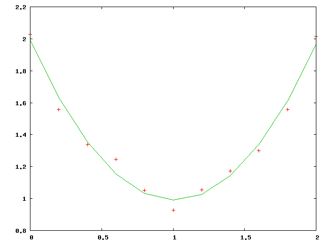
printf "set term gif\nset output\nplot 'poly.out' using 1:2 with points notitle,\
 'poly.out' using 1:3 with lines notitle\n" | gnuplot > poly.gif

rm poly.out

# the points are the original noisy data,
# the line is the polynomial approximation to the data

% ./poly.sh

poly.html